
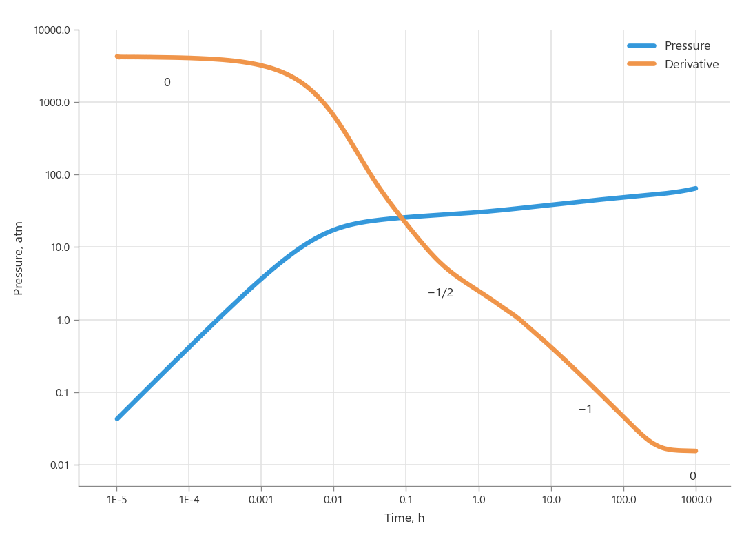
Take a look at the synthetic plot below. An experienced well test engineer will say almost immediately that it most likely shows a horizontal well with wellbore storage and boundary effects.
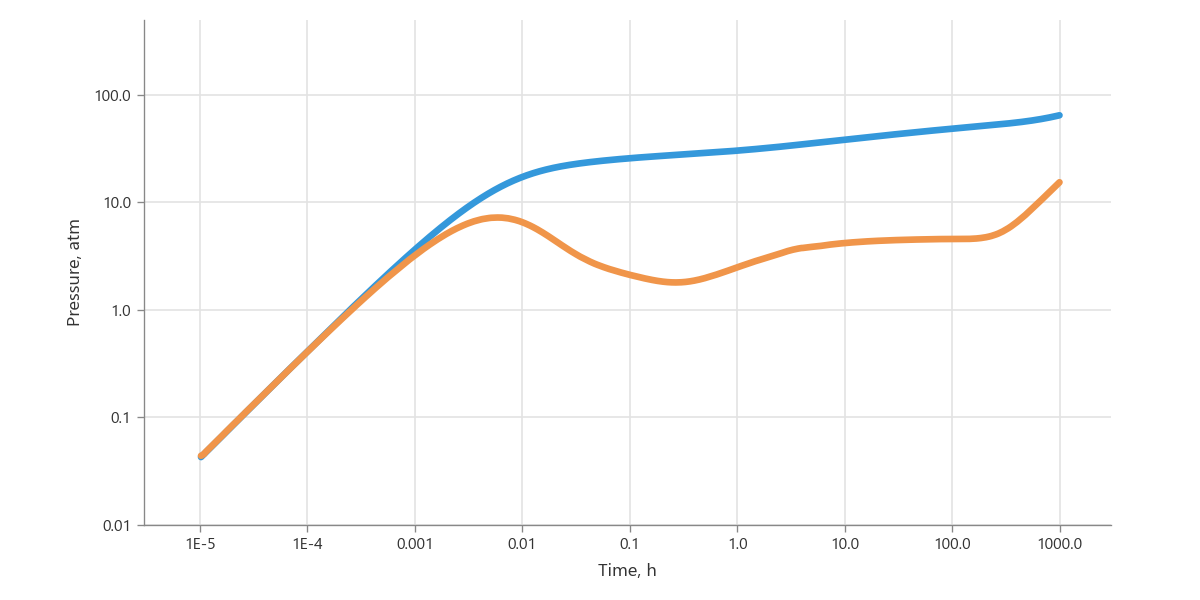
This kind of reading is possible thanks to the diagnostic signatures visible on the plot. The unit slope at the start corresponds to wellbore storage. The 1/2 slope in the middle points to linear flow. The horizontal plateau means radial flow. The unit slope at the end reveals the influence of reservoir boundaries. All of this comes together into a single picture, and the engineer makes a conclusion.
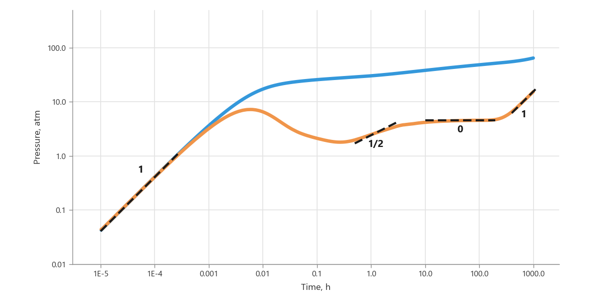
These are well-known patterns, and people usually memorize them. But they are not a convention or an agreement. They are a regularity rooted in the physics of the process and revealed by carefully chosen mathematical tools. In this article we take apart one such tool, the diagnostic plot, so that we understand not only how to use it but also why it works.
Where the powers come from
Look at the pressure curve below. We have deliberately removed its axes. Can you tell from its shape alone what kind of record it is: an hour, a week, or a year?
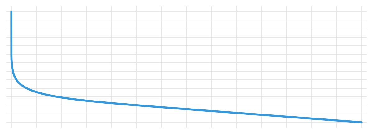
There is no way to guess. A pressure curve is built so that its shape does not reveal the time scale. It could be a segment spanning a day or a segment spanning a year: it all depends on the properties of the system, which set the scale.
This is no accident. If the shape of a curve does not change when the time axis is stretched, the dependence has no intrinsic scale. Only a power function has this property, along with its limiting case, the logarithm. Any other dependence has a scale built into it: a sine wave has a period, an exponential has a decay time. Stretch the axis, and the shape changes.
So in the flow equations, pressure must depend on time through a power. Let's check this against the main flow regimes:
| Flow regime | Equation | Time dependence | Exponent |
|---|---|---|---|
| Wellbore storage | $\Delta p = \dfrac{qB}{C}\, t$ | linear | 1 |
| Linear | $\Delta p = \dfrac{qB}{h\, x_f} \sqrt{\dfrac{\mu t}{\phi c_t k}}$ | square root | 1/2 |
| Bilinear | $\Delta p = \dfrac{qB\mu}{h \sqrt{k_f w}} \left(\dfrac{t}{\phi \mu c_t k}\right)^{1/4}$ | fourth root | 1/4 |
| Spherical | $\Delta p = \dfrac{qB\mu}{k_s r_s} - \dfrac{qB\mu \sqrt{\phi \mu c_t}}{k_s^{3/2}}\, t^{-1/2}$ | inverse square root | −1/2 |
| Closed reservoir | $\Delta p = \dfrac{qB}{\phi c_t h A}\, t + b$ | linear | 1 |
And indeed: no matter what these equations are made of, in every case pressure depends on time through a power. And these powers suspiciously match the slopes we saw on the diagnostic plot. The match is no coincidence, and to see the connection we need one more mathematical tool.
The logarithm turns a power into a slope
That tool is the logarithm. Recall the property from school: an exponent inside a logarithm can be brought out in front as a factor.
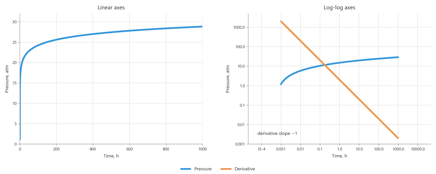
Let's see what this means on a plot. Take a simple power function $\Delta p = 2\sqrt{t}$, that is $2\,t^{1/2}$, and plot it twice: on linear axes and on logarithmic axes.
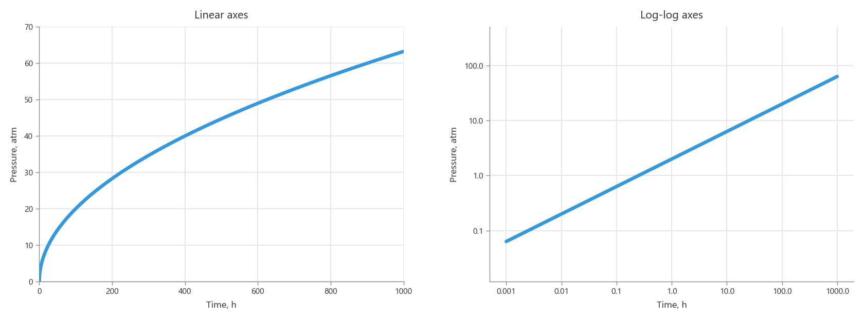
On linear axes it is a curve: it rises steeply at first and gradually flattens out. On logarithmic axes the very same function becomes a straight line. This is how the logarithm visibly straightens a power law: the exponent brought out in front becomes the slope of the line.
Our equations on a log-log plot
Let's return to the table of flow regimes. We strip the physics out of the equations and keep only their structure: all reservoir and well parameters are lumped into constant coefficients $a$ and $b$. Then we take the logarithm of each equation.
| Flow regime | Equation | After taking the logarithm |
|---|---|---|
| Wellbore storage | $\Delta p = a\, t$ | $\log \Delta p = \log a + \log t$ |
| Linear | $\Delta p = a\, t^{1/2}$ | $\log \Delta p = \log a + \frac{1}{2} \log t$ |
| Bilinear | $\Delta p = a\, t^{1/4}$ | $\log \Delta p = \log a + \frac{1}{4} \log t$ |
| Spherical | $\Delta p = b - a\, t^{-1/2}$ | $\log \Delta p = \log \left(b - a\, t^{-1/2}\right)$ |
| Closed reservoir | $\Delta p = a\, t + b$ | $\log \Delta p = \log \left(a\, t + b\right)$ |
The first three equations are pure powers. The logarithm takes them apart easily: the exponent moves to the front and becomes the slope, while everything related to the reservoir goes into $\log a$ and only shifts the line up or down. On a log-log plot we get clean straight lines with slopes of 1, 1/2, and 1/4.
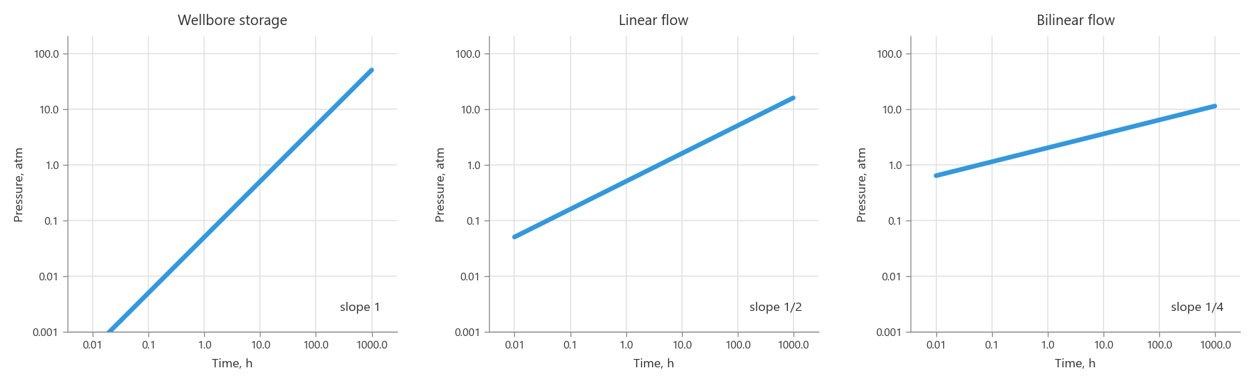
The last two equations don't work out this way. In them a constant term $b$ is added to the power, and the logarithm of a sum does not split into a sum of logarithms. The power stays locked inside the parentheses, and no straight line appears.
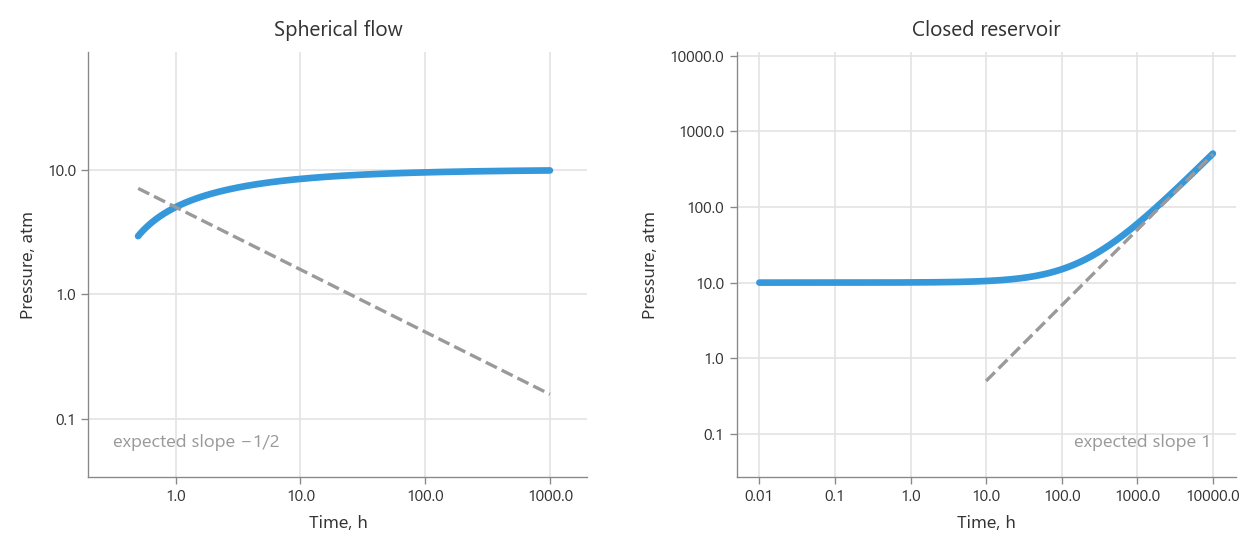
In spherical flow the constant dominates: pressure simply levels off, and the −1/2 slope does not show up on the plot at all. In a closed reservoir the constant interferes less: the unit slope does appear, but late and gradually, with no clear onset. To solve this problem, we turn to the derivative.
Getting rid of constants by differentiation
The derivative has exactly the property we need: a constant term vanishes under differentiation. Let's differentiate each equation and take the logarithm again:
| Flow regime | Equation | Derivative | After taking the logarithm |
|---|---|---|---|
| Wellbore storage | $\Delta p = a\, t$ | $\dfrac{d\Delta p}{dt} = a$ | $\log \dfrac{d\Delta p}{dt} = \log a$ |
| Linear | $\Delta p = a\, t^{1/2}$ | $\dfrac{d\Delta p}{dt} = \dfrac{a}{2}\, t^{-1/2}$ | $\log \dfrac{d\Delta p}{dt} = \log \dfrac{a}{2} - \dfrac{1}{2} \log t$ |
| Bilinear | $\Delta p = a\, t^{1/4}$ | $\dfrac{d\Delta p}{dt} = \dfrac{a}{4}\, t^{-3/4}$ | $\log \dfrac{d\Delta p}{dt} = \log \dfrac{a}{4} - \dfrac{3}{4} \log t$ |
| Spherical | $\Delta p = b - a\, t^{-1/2}$ | $\dfrac{d\Delta p}{dt} = \dfrac{a}{2}\, t^{-3/2}$ | $\log \dfrac{d\Delta p}{dt} = \log \dfrac{a}{2} - \dfrac{3}{2} \log t$ |
| Closed reservoir | $\Delta p = a\, t + b$ | $\dfrac{d\Delta p}{dt} = a$ | $\log \dfrac{d\Delta p}{dt} = \log a$ |
The constant is gone, and now all five derivatives are pure powers. On a log-log plot each of them becomes a straight line.
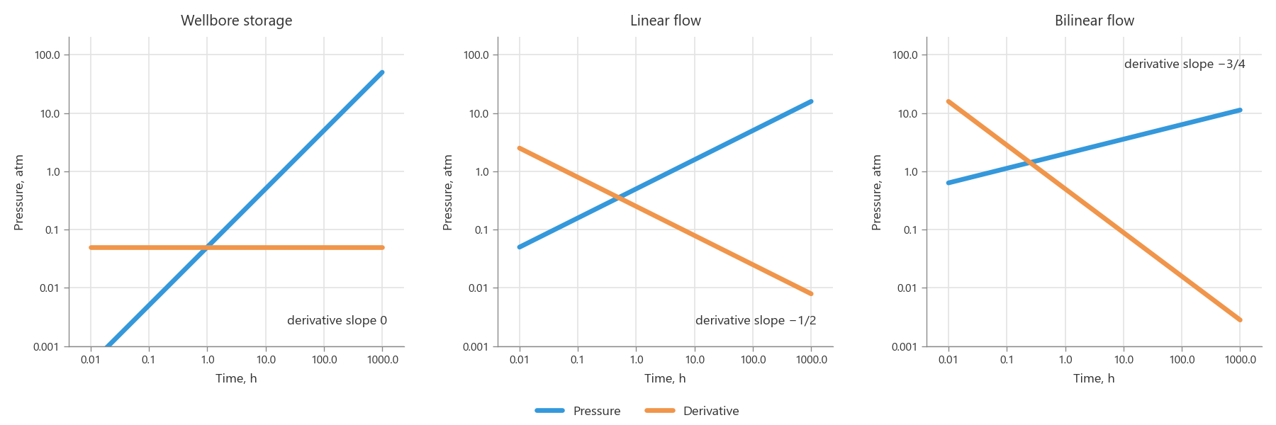
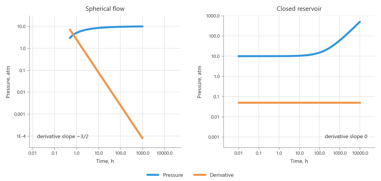
The derivative has solved the problem with spherical flow and the closed reservoir.
One more regime remains, which we have deliberately skipped so far: radial flow, one of the most important in well testing. Its equation looks like this:
Simplifying it the same way as the others, we get:
We skipped this case earlier because it is the limiting case: the dependence here is logarithmic, not a power. Taking the logarithm does not straighten such a curve; it stays bent on both linear and logarithmic axes. But the derivative handles it as well:
Once again a pure power, and on a log-log plot it becomes a straight line with a slope of −1.
Now we have straight lines for all six regimes, but this solution comes at a price. The derivative lowers the exponent by one, so its slopes do not match the slopes of the pressure itself. Linear flow now gives −1/2 instead of 1/2, and bilinear flow gives −3/4 instead of 1/4. And radial flow, the most important of them all, ends up with an unremarkable slope of −1.
On the whole, this works. If we plot the complex example from the beginning of the article, the regimes can in principle be told apart on the derivative, and over time one can get used to this look.
However, there is one more mathematical trick up our sleeve. It makes the picture noticeably better and gives the plot the look engineers are used to.
The Bourdet derivative: differentiating with respect to the logarithm of time
We will differentiate with respect to the logarithm. The idea is simple: since we look at the data as a function of the logarithm of time, it makes sense to differentiate along that same axis. This derivative was proposed by Dominique Bourdet in the early 1980s and has carried his name ever since:
Since $d \ln t = \dfrac{dt}{t}$, in practice it is very simple to compute: it is the ordinary derivative multiplied by time:
The factor $t$ makes up for what the ordinary derivative took away. For a power function this is immediately clear:
The ordinary derivative lowered the exponent by one, and multiplying by $t$ restored it. The function remains the same power; only the constant factor has changed.
With the logarithm it gets even more interesting:
Time disappears entirely, leaving a constant. Let's see what this gives for all six regimes:
| Flow regime | Equation | Bourdet derivative | After taking the logarithm | Slope |
|---|---|---|---|---|
| Wellbore storage | $\Delta p = a\, t$ | $\Delta p' = a\, t$ | $\log \Delta p' = \log a + \log t$ | 1 |
| Linear | $\Delta p = a\, t^{1/2}$ | $\Delta p' = \dfrac{a}{2}\, t^{1/2}$ | $\log \Delta p' = \log \dfrac{a}{2} + \dfrac{1}{2} \log t$ | 1/2 |
| Bilinear | $\Delta p = a\, t^{1/4}$ | $\Delta p' = \dfrac{a}{4}\, t^{1/4}$ | $\log \Delta p' = \log \dfrac{a}{4} + \dfrac{1}{4} \log t$ | 1/4 |
| Radial | $\Delta p = a \ln t + b$ | $\Delta p' = a$ | $\log \Delta p' = \log a$ | 0 |
| Spherical | $\Delta p = b - a\, t^{-1/2}$ | $\Delta p' = \dfrac{a}{2}\, t^{-1/2}$ | $\log \Delta p' = \log \dfrac{a}{2} - \dfrac{1}{2} \log t$ | −1/2 |
| Closed reservoir | $\Delta p = a\, t + b$ | $\Delta p' = a\, t$ | $\log \Delta p' = \log a + \log t$ | 1 |
All six regimes give straight lines. Note that wherever the pressure itself has a slope, the derivative has the same one.
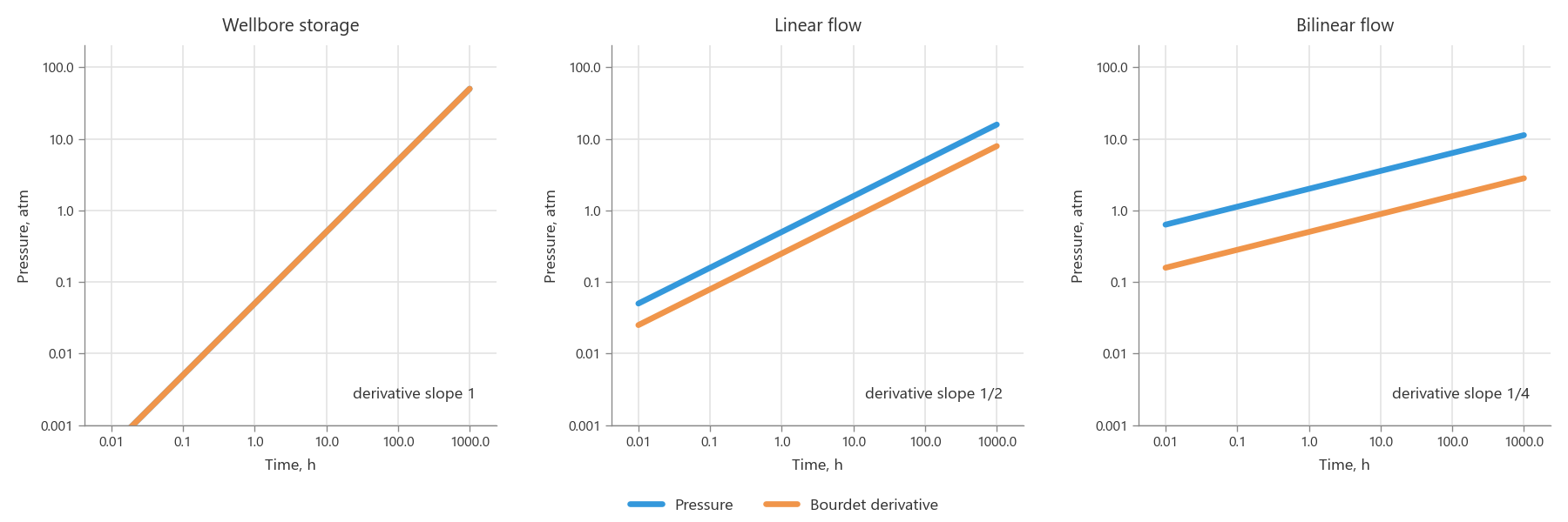
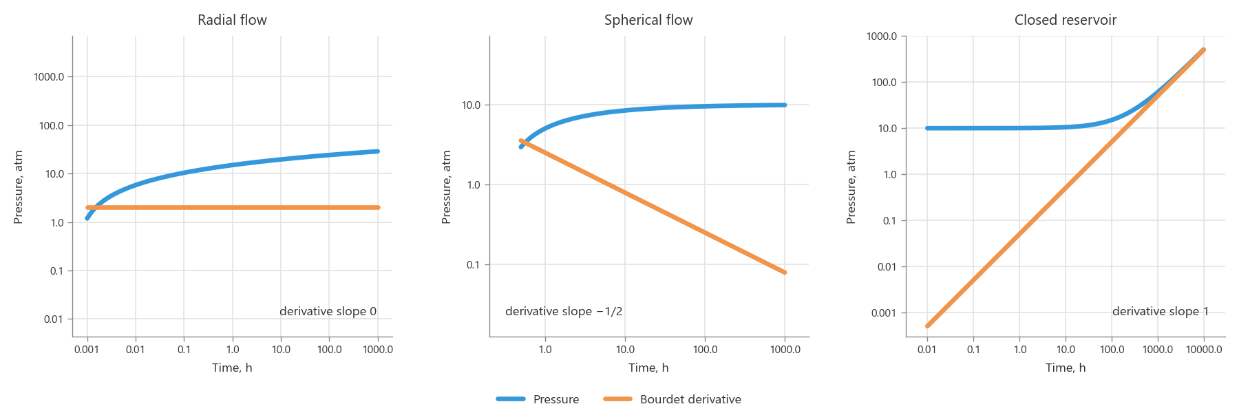
Compared with the ordinary derivative, the advantage comes on several fronts at once:
- Pressure and derivative slopes match. For pure power-law regimes the derivative runs parallel to the pressure, which gives an extra diagnostic signature.
- Radial flow becomes a horizontal plateau. The most important regime gets the most recognizable signature on the plot.
- The derivative is measured in the same units as pressure. Both curves are plotted on the same axes and in the same range of values, so they can be compared with each other.
The size of the difference is best seen on the complex example. On the left is the synthetic example from the beginning of the article with the ordinary derivative; on the right, with the Bourdet derivative:
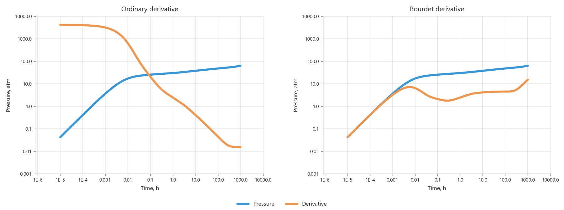
On the left the regimes can be told apart, but the plot is awkward to read. The derivative slopes are mostly negative and bear no relation to the pressure slopes, and radial flow looks like an ordinary decline that gets lost among the other regimes and transitions. On the right the lines are simpler and clearer, and the derivative runs parallel to the pressure in places, so the plot is much easier to read.
Conclusion
To wrap up, let's briefly retrace the whole path. The pressure function in a reservoir has no intrinsic time scale, so each flow regime is described by a power law. The logarithm turns the exponent into the slope of a straight line. The derivative removes the constants that got in the way of the logarithm. The Bourdet derivative puts the exponents back in place and makes the plot easier to read.
None of these steps is accidental. Each mathematical trick removes a specific obstacle left by the previous one. As a result, the diagnostic plot turns out to be not a set of conventions to memorize but a tool built so that reservoir physics shows up in it through simple geometric signatures an engineer can recognize.
Now, looking at a diagnostic plot, you can see behind its shape not just familiar patterns but the physics of what is happening in the reservoir. Familiar signatures will add up to a clear physical picture, and unfamiliar ones will spark curiosity rather than confusion: why does the plot look exactly like this, and what physical process lies behind it?
Instead of simply recognizing familiar shapes, the engineer begins to understand their causes, ask questions, and dig deeper into what is going on. And that is a whole different level of perception and understanding: the plot stops being a picture to recognize and becomes a way to see the physics of the reservoir.