PBU Analysis in SiamWellTest

Goal. Walk through a simple end-to-end pressure build-up (PBU) interpretation case in SiamWellTest and show the program's main capabilities, from setting up the diagnostic plot to the final reservoir parameters.

Audience. This document is intended for two groups of readers:

• well test engineers: see what SiamWellTest can do and what the familiar interpretation workflow looks like in it;
• petroleum engineers from other disciplines: get a general idea of how PBU tests are interpreted and where the reservoir parameters in well test reports come from.

What we do. Using a single PBU as an example, we go through the full interpretation cycle:

1. Setting up the diagnostic plot: decimation and smoothing.
2. Analyzing the diagnostic plot and identifying flow regimes.
3. Manually matching an initial guess.
4. Finding the best solution with the optimizer.
5. Recording the results.

The data for this case have been prepared in advance. Preparation of pressures, rates and PVT properties is covered in other cases, so we will not repeat it here.

Input data

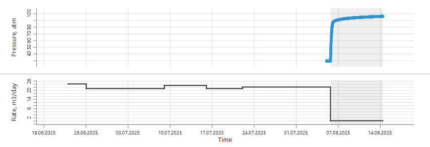
For this case we take a typical test of a low-rate oil well: a PBU recorded by the ESP downhole gauge and the rate history from the production report. The data were prepared in advance in the data preparation module: the pressure is loaded, the production periods are aligned with the pressure record, and the shut-in time is matched with the start of the PBU.

Pressure

Pressure was recorded by the downhole gauge at the pump intake. The record covers about 15 hours of production, followed by a shut-in on Aug 5, 2025 at 15:24 and almost 9 days of pressure build-up. During the PBU the pressure rose from about 29 to 96 atm.

Parameter	Value
Source	ESP downhole gauge
Recording period	Aug 5, 2025 – Aug 14, 2025
Sampling rate	5 s
PBU duration	≈ 210 h

Rates

Rates were taken from the production report. The production history before the shut-in is described by five flow periods with rates from 21 to 24 m³/d; the last period is 22 m³/d. The rate is assumed constant between records.

Parameter	Value
Source	Production report
Period	Jun 23, 2025 – Aug 14, 2025
Flow periods	5 production periods + PBU
Rate	21–24 m³/d

Reservoir and fluid parameters

Fluid properties were calculated separately in the PVT module and transferred to the analysis. Net thickness and porosity are taken from geological data, and the wellbore radius from the well design.

Parameter	Value
Wellbore radius, rw	0.108 m
Porosity, φ	0.18
Net thickness, h	8.6 m
Formation volume factor, B	1.2858 m³/m³
Viscosity, μ	0.760 cP
Total compressibility, ct	2.03·10⁻⁴ atm⁻¹

Setting up the diagnostic plot

Working with a PBU starts with choosing the decimation and smoothing coefficients. They are adjusted with sliders, and the diagnostic plot is rebuilt interactively. This makes it easy to tune the parameters by eye instead of trying values blindly.

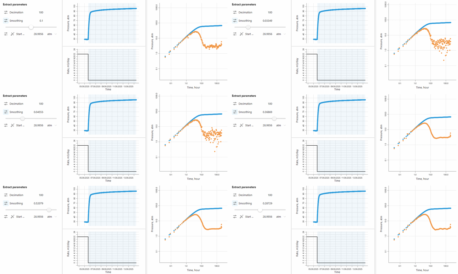
Decimation sets the number of points per log cycle. Fewer points mean less noise but also fewer details. More points give a more detailed curve. Usually 100 points per log cycle is enough; beyond that, no new useful details appear.

Smoothing sets the window width used to calculate the derivative. A smaller window distorts the data less, but the derivative stays noisy. A larger window makes the plot easier to read but distorts the shape of the curve more. We settle on 0.28: the late-time noise disappears while the shape of the curve is preserved.

Entering input data

After the derivative is calculated, SiamWellTest opens the analysis workspace: input data, plots and results. Reservoir and fluid parameters are entered in the left panel, in the "Input parameters" section: wellbore radius, porosity, thickness, formation volume factor, viscosity and compressibility.

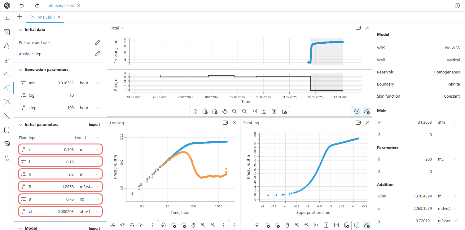
Three plots are located in the center:

• History — pressure and rate history on a single time axis, with the PBU interval highlighted. It is used to check how the model reproduces the historical data.
• Log-log — the diagnostic plot: pressure change and derivative. The main plot for identifying flow regimes.
• Semi-log — pressure versus superposition time. Used to verify the radial flow regime and to estimate permeability from the slope of the straight line.

The results panel is on the right. We will come back to it once the analysis is finished and we move on to reviewing the results.

Diagnostic plot analysis

We move on to the log-log plot and identify the flow regimes. They determine which model we will match. Two regimes stand out clearly on the plot.

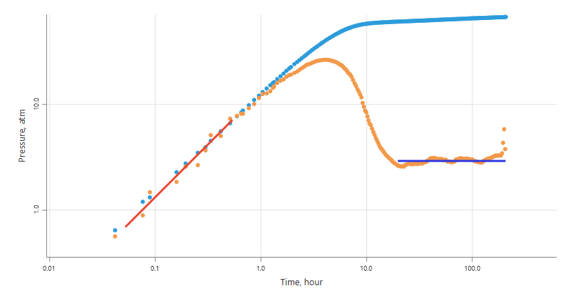
Wellbore storage (WBS). At early times, up to about 0.5 h, the pressure change and the derivative coincide and lie on a unit-slope straight line (red line). During this period the reservoir response is not yet visible: after a change in the well's rate, the sandface flow differs from the surface rate due to fluid compressibility in the wellbore or a changing liquid level. The position of this line determines the wellbore storage coefficient.

Transition period. Then the derivative departs from the pressure change, forms a hump peaking at about 3–4 h, and drops sharply. The height of the hump is related to the skin factor: the higher the hump, the larger the skin.

Radial flow. From about 20 to 200 h the derivative reaches a horizontal plateau (blue line). This is radial flow in an infinite-acting reservoir. The plateau lasts almost a full log cycle, so the regime is identified reliably. Its level determines the permeability.

The rise of the last few points is an end effect of the derivative calculation at the end of the record. We do not treat it as a boundary signature.

There are no signs of boundaries, reservoir heterogeneity or completion effects on the plot. So we choose a simple model:

• wellbore storage — constant;
• well — vertical;
• reservoir — homogeneous;
• boundaries — infinite;
• skin factor — constant.

Manual matching of the initial guess

The optimizer works more reliably when it starts from a point close to the solution. So we first match the model by hand. Parameters are changed with sliders in the "Parameters" panel, and the model curve on the log-log plot is rebuilt immediately.

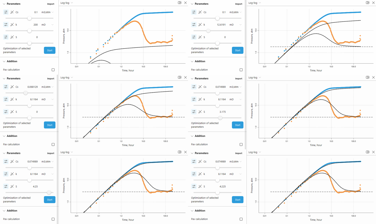
Each parameter has its own zone of influence on the plot, so it is convenient to match them one at a time:

1. Permeability k — move the model derivative plateau down or up to the level of the data plateau.
2. Wellbore storage coefficient Cs — shift the model unit-slope line onto the early-time points.
3. Skin factor S — adjust the height of the hump in the transition period.

The purpose of this step is to provide an initial guess so that the optimizer works faster and more accurately.

Refining the solution with the optimizer

Next we turn on regression. In the "Regression settings" window we select the parameters to optimize and set a search range for each. Permeability is determined confidently from the radial flow plateau, so we do not optimize it. We optimize Cs and S over evenly selected points of the diagnostic plot.

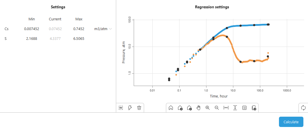
We click "Calculate". The optimizer finds the parameters for which the selected model best describes the data.

Results

Parameter	Value
Permeability, k	8.12 mD
Skin factor, S	4.24
Wellbore storage coefficient, Cs	0.068 m³/atm
Initial reservoir pressure, Pi	100.85 atm
Transmissibility, kh/μ	91.8 mD·m/cP
Diffusivity, χ	0.029 m²/s
Radius of investigation, Rinv	265 m

Additionally: changing wellbore storage

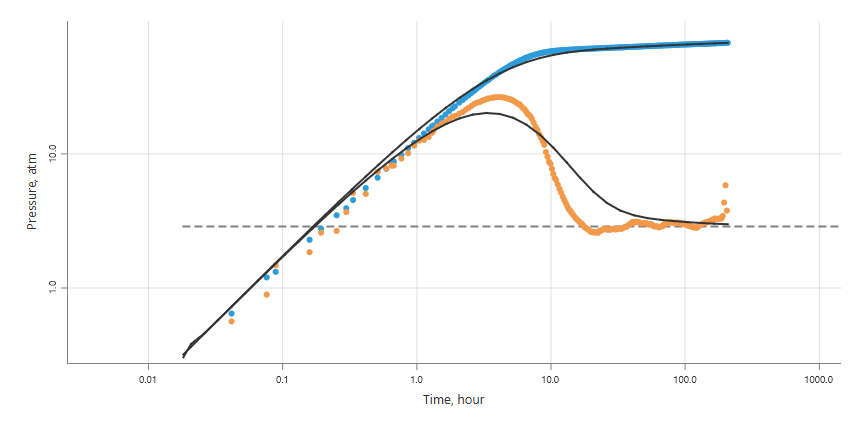
The model with classic wellbore storage describes the data well overall, but in the transition period the shape of the hump differs slightly from the model. Let's try the Hegeman changing wellbore storage model. In this model the wellbore storage coefficient changes over time, from the initial value Cf to the final value Cs, and the characteristic transition time is set by the parameter tf.

We change the wellbore storage type in the model panel and repeat the matching: first by hand, then with the optimizer.

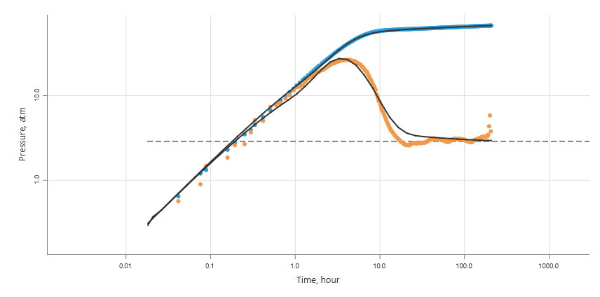
The model fits the data noticeably better, especially in the transition zone. At the same time, the main reservoir parameters remained practically unchanged.

Parameter	Classic WBS	Changing WBS (Hegeman)
Permeability, k	8.12 mD	8.12 mD
Skin factor, S	4.24	4.24
Initial reservoir pressure, Pi	100.85 atm	100.86 atm
Wellbore storage coefficient	Cs = 0.068 m³/atm	Cf = 0.070 → Cs = 0.033 m³/atm
Transition time, tf	—	9.2 h

Essentially this is a cosmetic refinement: it improves the match with the data but does not change the conclusions about the reservoir. Such a check is useful to make sure that permeability and skin do not depend on how the wellbore is described.

Results review

Permeability — 8.1 mD. The value is low but expected for this well: at a rate of 22 m³/d the drawdown is about 72 atm. This is a realistic value for a producing formation. It should be finally assessed against field data: core, well logs, and test results from offset wells.

Skin factor — 4.2. The near-wellbore zone is damaged. The cause needs to be investigated separately: history of well kills and workovers, deposits, perforation quality. If the skin can be reduced, the well will be able to produce the same rate at a lower drawdown or a higher rate at the same drawdown.

Reservoir pressure — 100.9 atm. This is the extrapolated pressure. We did not see any boundaries on the plot, so we do not calculate the average reservoir pressure. The obtained value accounts for the production history of the five flow periods before the shut-in. Since the reservoir in the model is infinite, with an infinitely long shut-in the pressure would reach exactly this value. The pressure refers to the gauge depth. To compare it with other wells, it needs to be corrected to a common datum.

Wellbore storage — 0.068 m³/atm. This is a typical value for artificially lifted wells. The large volume of the tubing and annulus and the rising liquid level after shut-in result in a high wellbore storage coefficient. The Hegeman model shows that wellbore storage is most likely changing: after about 9 hours the coefficient halves, from 0.070 to 0.033 m³/atm. The most likely reason is a change in the storage mechanism. Right after shut-in, the inflow goes into raising the liquid level in the wellbore. Once the level reaches the wellhead, only fluid compression remains, and wellbore storage decreases.

Conclusion

In this case we went through the full PBU interpretation cycle for a low-rate well in SiamWellTest: from prepared data to the final reservoir parameters and their review.

The entire interpretation was performed in a single module:

• The diagnostic plot is set up with the decimation and smoothing sliders, and the result is visible immediately.
• Flow regimes on the log-log plot are read unambiguously: wellbore storage at early times and radial flow for almost a full log cycle.
• The initial guess is matched by hand: each parameter has its own zone of influence on the plot.
• The optimizer refines the solution within the specified ranges.

This is the basic scenario that most interpretations start with. In the following cases we will look at tests with complex flow regimes and models.